The problem of sampling rule in Support Vector Machine raised in the discussion when I was in the course Advanced Remote Sensing.
The quality of training sample has deterministic influence to the accuracy of supervised classification methods. A properly designed sampling rule plays a substantial role in yielding an informative training sample set. The design of sampling strategy depends on both the characteristics of objects of interest and the applied classification methods.
Support Vector Machine (SVM) is an increasingly popular classification method for remote sensing image both in industry and research. As for the theory and concept of SVM, there have been many introductory articles such as [Roemer`s blog](http://rvlasveld.github.io/blog/2013/07/12/introduction-to-one-class-support-vector-machines/). Because support vectors are selected from training samples for maximizing the margin between classes, quality of sample set will decide the effectiveness of the hyperplane and affect the performance of the classifier.
In brief the mechanism of SVM is very different from traditional methods like Maximum Likelihood Classification. Here comes the question: Does the sampling rule used in traditional methods also work for SVM? How does the sampling rule affect the SVM classification result?
Experiment
To answer this question, I would like to set up a scenario for the classification experiment. In this case, I choose to perform a cloud detection based on Landsat 8 OLI image for two reasons:
It is a most basic binary classification.
Cloud detection could be very challenging because thin cloud is very difficult to detect in many situations.
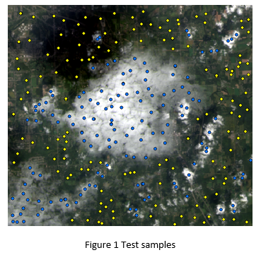
I use an image with both thick cloud and thin cloud in order to increase the difficulty of classification (See Figure 1). Band 2 to 7 are used and the SVM classifier in ENVI is utilized with default configuration. Four hundred pixels are randomly picked up as test sample: half of them are cloud (blue points) and the others are ground objects (yellow points).
Sampling Rules
I am particularly interested in three sample rules.
- Stratified random sampling
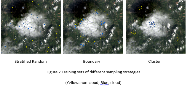
This is a classic sample rule. Its idea is to randomly select training samples of one class from the sample pool of that class. The sample size of each class could be a fixed number or proportional to the size of sample pool of that class.
- Cluster sampling
However, in practice random sampling is sometimes difficult to achieve, especially when the sample is selected by hand or a semi-automatic method. The sample pixels generally tend to be more clustering than random. (it is actually what we do in the ENVI class: drag a region of interest and treat it as sample set)
- Boundary sampling
Its basic idea is that support vectors are likely also located near the geographical boundary of two classes. Although pixels located around geographic boundaries might contain spectral information of both classes to some extent, Foody and Mathur (2006) suggested that mixing pixels at two sides of ground object boundary could be highly effective in SVM even the sample size was very smaller. They considered this approach as a competitive alternative of conventional sampling strategy.
So I select three training sets based on above sampling rules (See Figure 2).
Training set in feature space
While using the SVM, we hope that our training samples are located near the boundary of classes in the feature space. Figure 3 shows how samples in three training sets, as well as the test set, scatter at a feature space (red band vs. NIR band).
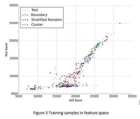
Cloud has high reflectance in both red band and near infrared band, however, the reflectance of ground objects (most are vegetation) is low in red band and high in near infrared band. Due to the reflectance difference, samples in the feature space apparently belong to two distinct groups: cloud and ground objects. As shown in Figure 3, the distribution of samples in different training sets are totally different. Boundary sampling produced samples located near the boundary of two classes. Samples generated with stratified random sampling could better represent the overall characteristics of two classes. Clustering sampling within high confidence area would generate samples also clustering in the feature space.
Result
The classification results are shown in Table 1 and Figure 4.
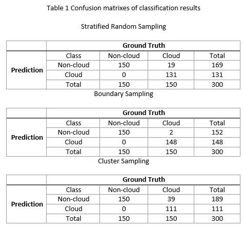
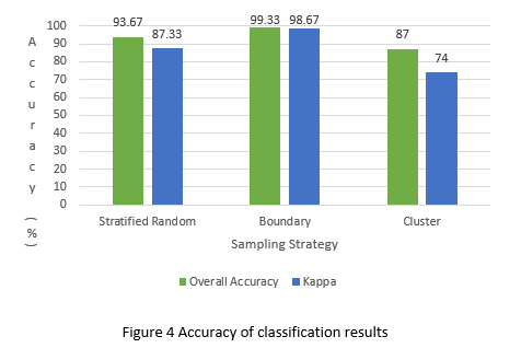
The results, as expected, indicate that boundary sampling is able to generate better training sample and contribute to higher classification accuracy, compared to the other two sampling strategies.
ALl trained classifiers are also applied to the whole study image. Classifier trained with boundary samples is very sensitive to the difference between cloud and non-cloud pixels. It will try to differentiate all mixing pixels and this could be too sensitive. Classifier trained by cluster samples only recognizes thick cloud on the image and ignores pixels with mixing spectral information. Classifier trained by stratified random samples takes a balance between them: neither too aggressive nor too conventional. For detailed discussion, please read my report (see link below).
Conclusion
Let’s get back to our initial questions and their answers.
- Does the sampling rule used in traditional methods also work for SVM?
Apparently the traditional stratified random sampling still works pretty well for the SVM classification. The classification accuracy in the experiment is about 90%, which is high enough for most situations.
- How does the sampling rule affect the SVM classification result?
If we can use the portion of boundary (mixing) pixels in the training set to define sampling rule, we are able to build a link among three sampling rules used above. As we include more boundary pixels into the training set, the classifier would become more sensitive and have a better performance in identifying mixing objects. However, high sensitivity could also increase the error rate while identifying mixing objects. There is a trade-off between high sensitivity and low error rate within the selection of sampling strategies.
There is no generally appropriate sampling rule for all situations. However, depending on the need of classification, there exits an appropriate sampling rule for specific situation. Therefore, it is not difficult to understand why the stratified random sampling is still the first choice in practical use. Though classifier trained stratified random sampling is expected to have fair performance, it is less likely to be trapped into the problem of overestimation and underestimation.
Link
This article is a simplified version of my project report. For more detail, please read my full report A Comparison of Sampling Strategies in SVM Classification.
Reference
[1] Foody, G. M. and A. Mathur (2006). “The use of small training sets containing mixed pixels for accurate hard image classification: Training on mixed spectral responses for classification by a SVM.” Remote Sensing of Environment 103(2): 179-189.